Learn SPSS in 15 minutes – step by step tutorial to get started with SPSS for data analysis

The Statistical Package for the Social Sciences, or IBM SPSS for short, is one of the most popular data analyses software around. Its popularity is due to how it makes it extremely easy to do basic and complex statistical analyses using a simple graphical user interface. This is unlike many other data analysis software that require that you to write complex code to do even the most basic of tasks.

SPSS is very popularly used in the academics, business and in many development organizations worldwide, so it goes without saying that investing your time into learning it is one of the best decisions you can make as far as your professional development is concerned.

In this SPSS training tutorial which has over 700,000 views on YouTube, I will walk you through the basics of SPSS from data entry to basic data analyses. Specifically, we will tackle how to create variables, how to enter data, how to analyze data using basic statistics and how to develop some basic charts.

The SPSS interface

The main interface of SPSS is called the Data Editor window. This is where most of the operations in SPSS take place – from creating variables to transforming the data and choosing analyses.

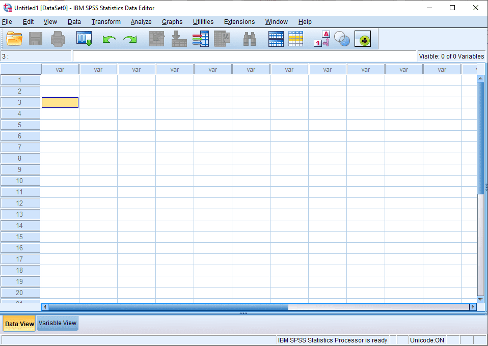
The data editor window is akin the Microsoft Excel spreadsheet – a huge table with rows and columns.

In SPSS the columns are the Variables. Think of the variables as the pieces of information you were collecting, or individual questions on a survey form.

The rows are known as cases – or individual respondents on a survey. This could be a single household in a household survey, or a single patient in a clinical study.

The data editor window is composed of 2 tabs – the data view and the variable view. The tabs used to switch between these views are located at the bottom-left of the window.

The data view is where you can view and edit the data.

The variable view is where you can define and edit the variables.

Getting data into SPSS

There are a multitude of ways in which data can be brought into SPSS. In this article, I will demonstrate how to define variables and enter data manually, as a way of bringing data into SPSS.

Defining variables in SPSS

To define variables, we first need to switch to the variable view on the data editor window. Do so by clicking on the Variable view tab at the bottom-left of the window.

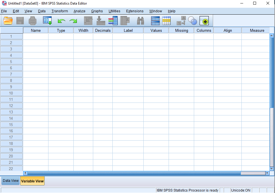
Here, we will have to define the characteristics of each of the variables such as the variable name, type, width and so on.

• Variable name – this is a name that will be used by the SPSS program to uniquely identify the variable. When defining the variable name, certain rules must be followed:
  • The name cannot contain spaces
  • The first character of the variable name cannot be a number
  • The name can only contain letters on the alphabet, numbers and the underscore (_)
• Variable type – the data type of the variable. These include the following:
  • Numeric – This is for variables whose values will be stored as numbers. This accounts for the majority of variables for most surveys. Numeric variables include variables that are:
    • Continuous e.g. Household size or household income
    • Categorical variables like Sex or Marital Status. The text values of these variables are stored as coded numbers where each number stands for a category within the variable. For example for the variable sex, we can assign 1 for Male and 2 for Female
  • Comma – A numeric variable whose values are displayed with commas delimiting every three places and displayed with the period as a decimal delimiter. An example of such variables is income.
  • Dot – Just like the Comma but using a dot instead of a comma to delimit every three places.
  • Scientific notation – A numeric variable whose values are displayed with an embedded E and a signed power-of-10 exponent. E.g. 5.634E-5 which translates to 0.00005634
  • Date: A numeric variable whose values are displayed in one of several calendar-date or clock-time formats. An example is date of birth.
  • Dollar – A numeric variable displayed with a leading dollar sign ($), commas delimiting every three places, and a period as the decimal delimiter. You can enter data values with or without the leading dollar sign.
  • Custom currency – A numeric variable whose values are displayed in one of the custom currency formats that you can define on the Currency tab of the Options dialog box. Go to Edit -> Options -> Currency to define the custom currencies.
  • String (text or alphanumeric) – A variable whose values are not numeric and therefore are not used in calculations. The values can contain any characters up to the defined length.
  • Restricted numeric – A variable whose values are restricted to non-negative integers. Values are displayed with leading zeros padded to the maximum width of the variable. E.g. if the width of the variable is 4, a value of 20 will appear as 0020.
• Width – The total number of characters for the longest response
• Decimals – The number of decimal places for the variable
• Label – The display name for the variable
• Values – This is where you set the list of values for categorial variables. For example, if you set the sex variable as numeric, you must set the codes and their corresponding values under the values dialog box which you can open by clicking the 3-dotted button
• Missing – You may define values as special missing values e.g. to distinguish between data that are missing because a respondent refused to answer (88: refused to answer) and data that are missing because the question didn’t apply to that respondent (99: not applicable). Data values that are specified as user-missing are flagged for special treatment and are excluded from most calculations
• Columns – The width of the data column for the variable measured in number of characters
• Align – Alignment of data in cells for that variable. The default alignment is right for numeric variables and left for string variables
• Measure – The measurement level for the variable. You can specify the level of measurement as scale (numeric data on an interval or ratio scale), ordinal, or nominal. Nominal and ordinal data can be either string (alphanumeric) or numeric.
  • Nominal. A variable can be treated as nominal when its values represent categories with no intrinsic ranking (for example, the department of the company in which an employee works). Examples of nominal variables include region, postal code, and religious affiliation.
  • Ordinal. A variable can be treated as ordinal when its values represent categories with some intrinsic ranking (for example, levels of service satisfaction from highly dissatisfied to highly satisfied). Examples of ordinal variables include attitude scores representing degree of satisfaction or confidence and preference rating scores.
  • Scale. A variable can be treated as scale (continuous) when its values represent ordered categories with a meaningful metric, so that distance comparisons between values are appropriate. Examples of scale variables include age in years and income in thousands of dollars.
• Roles: Some dialogs support predefined roles that can be used to pre-select variables for analysis. When you open one of these dialogs, variables that meet the role requirements will be automatically displayed in the destination list(s). Available roles are:
  • Input: The variable will be used as an input (e.g., predictor, independent variable).
  • Target. The variable will be used as an output or target (e.g., dependent variable).
  • Both: The variable will be used as both input and output.
  • None: The variable has no role assignment.
  • Partition: The variable will be used to partition the data into separate samples for training, testing, and validation.

Let’s take a look at one variable as an example – Interview ID:

1. In the first row of the Name column, type InterviewID
2. Press your Tab key to go to the type column. Here, click the 3 dotted button to open the Variable Type dialog box. Choose Numeric and click OK
3. Press your tab key to jump to width. Here we will leave the default as is.
4. Press TAB again to go to Decimals. Type 0 for the number of decimal places
5. Press tab to jump to Label. Here we will type the name of the variable in full the way we want it to look in our analysis output. So type Interview ID
6. Press TAB. The InterviewID variable will not have any assigned values. We will also not se missing values and we will leave the column width and alignment to default.
7. Tab up to the Measure column. We will choose Nominal

Let’s enter a few more variables

Name	Type	Decimals	Label	Values	Measure
Name	String	0	Name		Nominal
Gender	Numeric	0	Gender	1 – Male 2 – Female	Nominal
Age	Numeric	0	Age		Scale
Rice	Numeric	0	Did you eat Rice in the past 7 days?	1 – Yes 0 – No	Nominal

The Variable view will look like this:

Data Entry

Entering data in SPSS is very straightforward. If you have entered data in Excel before, you will be familiar with the SPSS interface and easily enter data.

First, switch to the data view using the tabs on the bottom-right corner of the data editor screen.

By default, we will be seeing the actual values we are entering in the data editor. For example, under the Gender column, when we type 1, we will also see 1. However, In most cases when you have variables with value sets, it will be great to see the labels instead. So, when we type 1, it should show us Male. For this to happen, turn on the Value Labels button on the toolbar at the top of the screen. – it says Value Labels.

Now enter the following data:

InterviewID	Name	Gender	Age	Rice
1	Peter	Male	15	Yes
2	Marian	Female	20	Yes
3	John	Male	18	No
4	James	Male	13	Yes
5	Peter	Male	18	Yes
6	Emily	Female	19	No
7	Erica	Female	22	No
8	Jean	Female	25	Yes
9	Jane	Female	22	No
10	Victoria	Female	26	No
11	Sean	Male	17	Yes
12	Ryan	Male	19	Yes
13	Kelvin	Male	22	Yes
14	Sangwani	Male	23	No
15	Robert	Male	22	Yes
16	Ralph	Male	18	Yes
17	Cicy	Female	19	No
18	Maggie	Female	25	Yes
19	Chifundo	Female	22	No
20	Sellina	Female	25	Yes

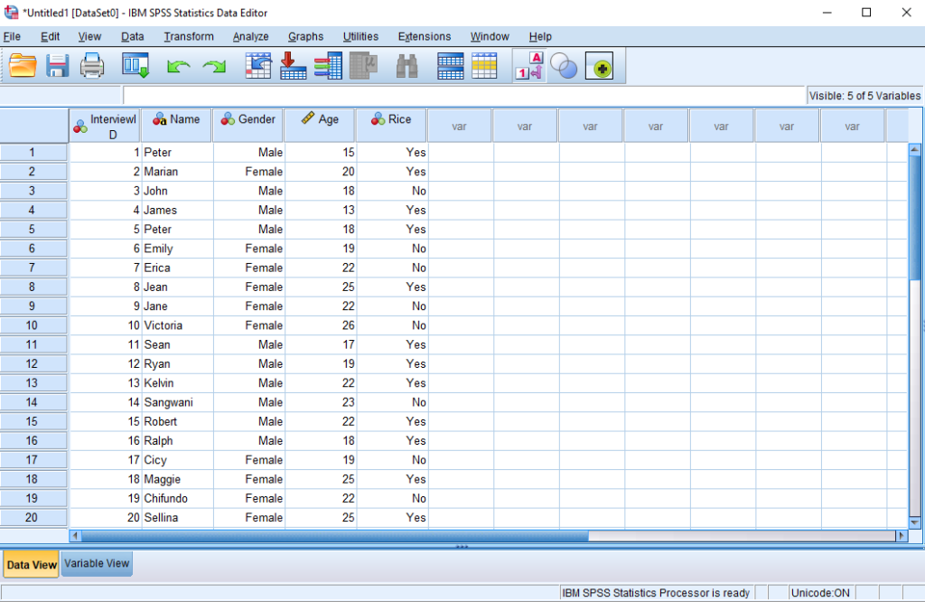
Your data will look like this:

Data Analysis

There are numerous kinds of data analyses available in SPSS and all of them are found under the Analyze option on the menu.

In this guide, we will look at basic descriptive statistics.

Analyzing categorical variables

Variables that were designated as ordinal or nominal are best analyzed using frequencies. Frequencies are simply the number of times a value appears in the data set. For example, we may be interested to know how many people were male and how many were female.

• Click on the Analyze item on the menu, point on Descriptive statistics and click Frequencies

• On the dialog box, Click and drag the Gender variable to the box on the right

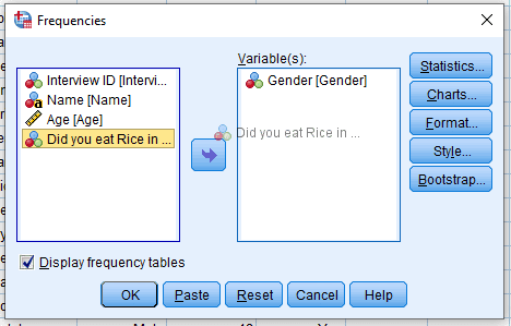
• Do the same for the “Did you eat Rice in the past 7 days?”
• Click the Charts button on the right of the dialog box
• Choose bar charts and click Continue

• Click OK

A new window called the Viewer will appear with the results of your analysis

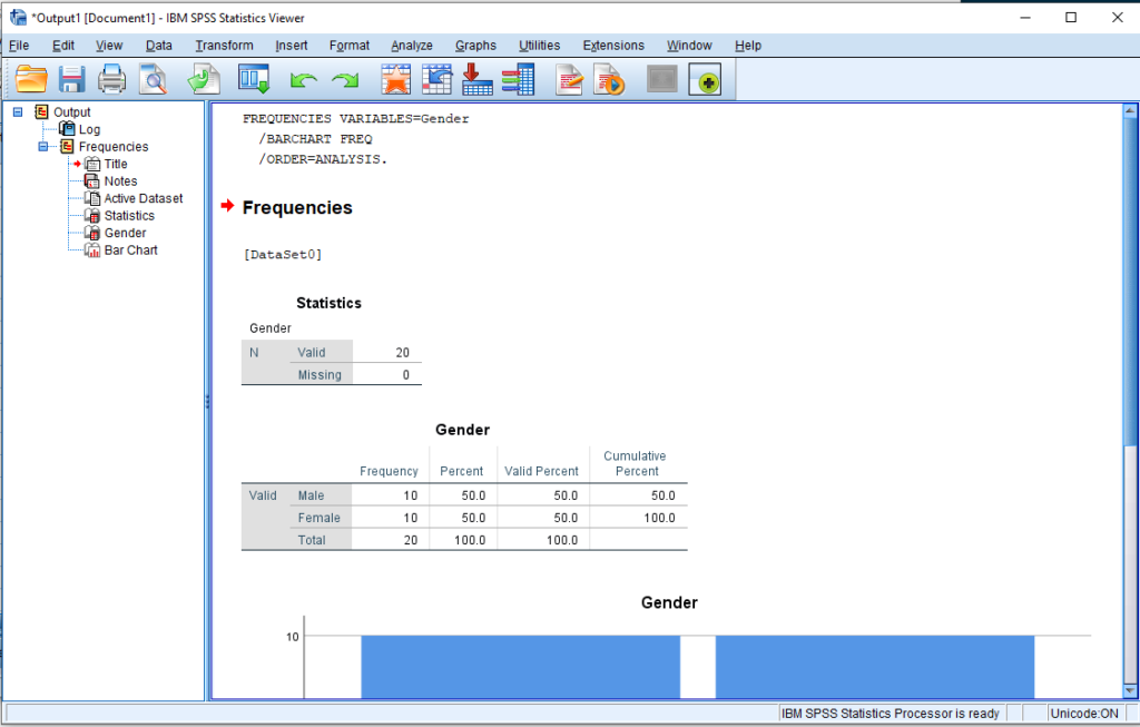
The first table in the output are the Statistics. Since we did not select any statistics, we only have 2 values: Valid and Missing.

• The Valid number represents the number of cases that have valid responses on the variable.
• The Missing number represents the number of cases that did not provide a valid response to the variable – either by leaving it blank or by providing a value that we defined as Missing in the variable view.

The second table is the Table of Frequencies.

• Frequency stands for the number of times the value appears in the data set.
• Percent is the frequency/count expressed as a percent out of the total number of cases in the data set
• Valid percent is the frequency/count expressed as a percentage out of the Valid cases – the number of people who actually gave a response on the variable. In most cases, this is the value that gets reported.
• The cumulative percent is the total percentage of the sample that has been accounted for up to that row; it can be computed by adding all of the numbers in the Valid Percent column above the current row.

To report the results from the table you can say:

There was a total of 20 respondents in the survey. Out of this, 10 were Male, and 10 others were Female – each representing 50% of the sample respectively.

To get the output to Microsoft Word for your reporting, just right-click on the output e.g. a chart or a table and select copy. In Microsoft Word, right click where you want the chart or table to go and select paste.

Analyzing continuous (scale variables)

The frequency table that we produced in the last analysis wont work well with variables that have many different data values, for example age. The result will simply be a long table of frequencies that doesn’t make any sense.

When we arrange the values of a variable in order from the lowest to the highest, we call this the frequency distribution.

To analyze scale variables, we first of all find the central point or average of the frequency distribution. We use the mean, the median or the mode for this. These 3 measures are known as measures of central tendency.

The measures of central tendency alone wont paint the full picture of what’s going on with the variable. Aside from observing the central point, we also need to know how the values vary within the variable. We do this using measure of variability also known as measures of dispersion. These include the range, variance and standard deviation.

• Back in the SPSS data editor window, click Analyze -> Descriptive Statistics -> Frequencies
• Click the Reset button at the bottom of the dialog box
• Move the Age variable to the box on the right by dragging and dropping
• Click the Statistics button
• Put checkmarks on Mean, Median, Std Deviation, Range, Minimum, Maximum and Quartiles

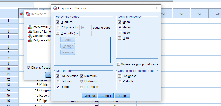
• Click Continue
• Click the Charts button
• Select Histogram and turn on “Show normal curve on histogram”
• Click Continue
• Turn off “Display Frequency Table” option at the bottom left of the Frequencies dialog box

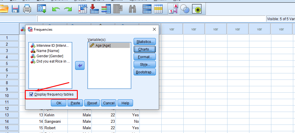
• Click OK

Once again, you will have your output appear in the Viewer window.

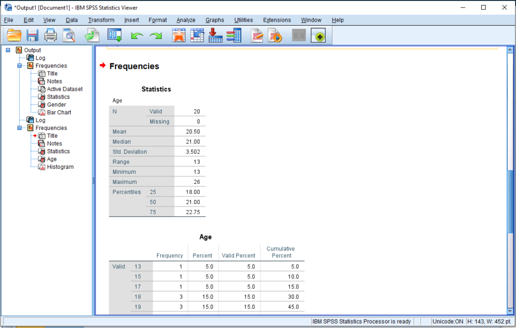
Once again we have our Table of Statistics. This time with more statistics – the ones we selected in the Statistics options dialog box

• Mean – The mean is found by adding all the numbers together and dividing by the number of values there is in the distribution.
• Median – The value is found by taking the number that is exactly on the middle of the distribution. in the case that the number of values is divisible by 2 as is the case with our data set (Valid=20), the mean of the 2 middle numbers is used.
• The standard deviation is the average of all differences between each value in the distribution and the mean. If the mean is the true center of the distribution, then the standard deviation shows on average how each value varies from it. If the difference is 0, then there are no differences between each value (in essence it means all cases had the same age). A standard deviation that is greater than 0 means there is more variability in the data set.
• The range is simply the difference between the largest value and the lowest value in the distribution.
• The percentiles show the value at which the said percent of values in the distribution lie. For example, he 25th percentile is a value at which 25% of the scores are below it.

Conclusion

The Statistical Package for the Social Sciences (SPSS) shines when it comes to ease of use when doing data analytics. With a great graphical user interface, IBM SPSS is easily the best choice for everyday data management and analysis.